Multi-hop Attention Graph Neural Networks

GAT中的attention运算只能关注节点相连节点表达，这种机制不考虑不直接相连但又有很重要信息的节点表达。

所以提出了多跳注意力图神经网络(MAGNA)，这是一种将多跳上下文信息融入到注意力计算的每一层的方法。

其将注意力分数分散到整个网络，相当于增加了每一层的GNN的“感受野”。

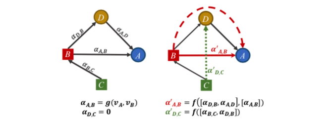
如左图，考虑A和D节点，普通的attention层只计算直接相连节点的注意力分数，如 $ \alpha{A,D} $ , 但如果C的信息很重要， $ \alpha{C,D}=0 $ 关注度却为0。并且，单个GAT层中A和D节点之间的运算只依赖于自己的表达，而不依赖于它们的图邻域上下文。其相当于每一层只关注了一阶邻居范围的感受野，虽然堆叠多层GNN可以扩大这个范围，但GNN层数一多就会有过平滑的问题。

再看右图，MAGNA 层的改进方法是

• 通过扩散多跳注意力捕捉 $ \alpha{D,C}’ $ 表达为 $ \alpha{D,C}’ = f([\alpha{B,C},\alpha{D,B}]) $
• 基于图邻接矩阵的权值，通过分散注意力来考虑节点之间的所有路径，从而增强图结构学习。MAGNA利用D的节点特征进行A和B之间的注意力计算，这意味着MAGNA中的两跳注意力是基于上下文的。

总之，GAT中的一跳注意机制限制了探索更广泛的图形结构与注意权重之间关系的能力。

本文提出了多跳注意图神经网络(MAGNA)，这是一种针对图结构数据的有效的多跳自注意机制。Magna使用了一种新颖的图形注意力扩散层(图1)，其中我们首先计算边上的注意力权重(用实心箭头表示)，然后使用边上的注意力权重通过注意力扩散过程计算断开的节点对之间的自我注意力权重(虚线箭头)。

方法

参数定义

图 $G =(V,E)$ , $E\in V\times V$ , V 节点集有 $N_n$ 个 ，E 边集有 $N_e$ 个

节点 v 到其类型的映射为 $ \phi: V \rightarrow \Tau $ , 边e 到其关系类型的映射 $\psi : E \rightarrow R$

节点的embedding : $X \in \mathbb{R}^{N_n\times d_n}$ , 边的embedding: $R\in \mathbb{R}^{N_r\times d_r}$

其中 $N_n = |V|, N_r=|R|$ , $d_n,d_r$ 是节点和边类型的embedding维度。

Embedding 的每行 $x_i = X[i:]$ 表示节点 $v_i (1\le i\le N_n)$ 的embedding ， $r_j=R[j:] , r_j(1\le j\le N_r)$

首先看一下MAGNA 模块的整体结构

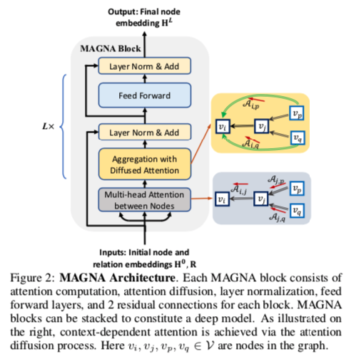
有点像Transformer block，现在GNN的包装越来越往Transformer based模型上靠了。

他传入节点和关系embedding，会首先经历一个对于每个节点的多头注意力层（这里和GAT一样），然后是注意力扩散、 Layer Norm、前向传播层和两个残差链接。

Multi-hop Attention Diffusion

Attention diffusion是每一层中用于计算MAGNA‘s的attention分数。首先第一阶段，计算每一条边上的attention分数。第二阶段，用扩散注意力计算多条邻居的注意力。

Edge Attention Computation.

在每一层 $l$ 处，为每个三元组 $(v_i，r_k，v_j)$ 计算矢量消息。 为了计算在 $l+1$ 层的表示，将关联的三元组的所有消息聚合成一条消息，然后使用该消息更新 $v_j^{l+1}$。

在第一阶段， 一个边 $(v_i,r_k,v_j)$ 的注意力分数是由以下计算而来：

$$s_{i,k,j}^{(l)} = LeakyRelu(v_a^{(l)} tanh(W_h^{(l)} h_i^{(l)} || W_t^{(l)}h_j^{(l)} || W_r^{(l)}r_k))$$

$ W_h^{(l)} , W_t^{(l)}\in \mathbb{R}^{d^{(l)}\times d^{(l)}} , W_r^{(l)}\in \mathbb{R}^{d^{(l)}\times d_r} , v_a^{(l)}\in \mathbb{R }^{1\times 3d^{(l)}}$ 可共享的可训练参数。

$h_i^{(l)}\in \mathbb{R}^{d^{(l)}}$ 是第 $l$ 层第 $i$ 个节点的embedding。 $h_i^{(0)} = x_i$

$r_k (1\le k \le N_r)$ 是可训练的第 $k$ 个关系类型的embedding

将上式应用到graph中的每一条边后，得到 attention score matrix $ S^{(l)}$:

$$S^{(l)}_{i,j} = \begin{cases} s_{i,j,k}^{(l)}, &\ (v_i,r_k,v_j)\ appears\ in\ G\\ \infty, &otherwise \end{cases}$$

随后，我们通过对得分矩阵 $S^{(l)}$ 执行逐行Softmax来获得注意力矩阵 $A^{(l)}_{i,j} = Softamax(S^{(l)})$

$A^{(l)}_{i,j}$ 就定义为在第 $l$ 层中当 从节点 $j$ 和 节点 $i$ 聚合消息时的关注值。

这里其实和GAT差不多 只是多了不同种边和节点。

Attention Diffusion for Multi-hop Neighbors

通过以下注意力扩散过程，在网络中将计算不直接连接的节点之间的注意力。

该过程基于1-hop 注意力矩阵A的幂 为：

$$A = \sum^{\infty}_{i=0}\theta_iA^i \ \ \ where \sum_{i=0}^{\infty}\theta_i = 1 \ and \ \theta_i \gt 0$$

其中 $\thetai$ 是 attention decay factor 并且 $\theta_i \gt \theta{i+1}$ ，

注意矩阵的幂 $A^i$ 给出了从节点 $h$ 到节点 $t$ 的长度为 $i$ 的关系路径的数量，从而增加了注意的感受野。

重要的是，该机制允许两个节点之间的注意力不仅取决于它们之前的层表示，而且还考虑到节点之间的路径，从而有效地在不直接连接的节点之间创建 attention shotcuts

在实现过程中，作者使用几何分布 (geometric distribution) $θ_i=α(1−α)^i$，其中 $α∈(0，1]$ 。

该选择基于the inductive bias ，即较远的节点在消息聚合中应该被较小的权重，并且具有到目标节点的不同关系路径长度的节点以独立的方式被顺序加权。

此外，请注意，如果定义$θ0=α∈(0，1] ，A_0=I$ ，则上面的公式。利用关注矩阵A和移动概率 $α$ ，给出了图上的Personal Page Rank。因此，扩散注意力权重 $A{i,j}$ 可以看作是节点 $j$ 对节点 $i$ 的影响。

同时对与目标节点关系路径长度不同的节点权重应该相互独立。因此，本文定义了基于特征聚合的graph attention diffusion：

$$AttDiff(G,H^{(l)}, \Theta) = A H^{(l)}$$

其中 $\Theta$ 为注意力参数集合。

Approximate Computation for Attention Diffusio

对于大图，公式（3）的计算开销巨大，而DAGCN需要通过 $AH^l$进行信息聚合，本文通过定义一个数列 $Z^K$, 当 $K \rightarrow \infty$时，该数列能收敛到$AH^l$的值：

$$Z^0 = H^L, Z^{k+1} = (1-\alpha)AZ^{(k)} + \alpha Z^0 \\ lim_{K\rightarrow \infty} Z^{K} = AH^{l}$$

证明请参考原文。上述的近似使得attention的复杂度保持在$O(|E|)$。很多真实世界网络具有小世界（small-world ）特征，在这种情况下，较小的K值就足够。对于具有较大直径的图，选择较大的K和较小 $\alpha$ 。

Multi-hop Attention based GNN Architecture

图2提供了可多次堆叠的MAGNA block 的架构概览。

Multi-head Graph Attention Diffusion Layer

在不同的视角联合关注来自不同表示子空间的信息。

$$\begin{equation}\begin{split} \hat H^{(l)} &= MultiHead(G, \hat H^{(l)}) =(||_{i=1}^M head_i) W_o \\ head_i &= AttDiff(G, \hat H^{(l)}, \Theta_i) \\ \hat H^{(l)} &= LayerNorm(H^{(l)}) \end{split}\end{equation}$$

方程中以递归的方式计算注意力扩散。增加了层归一化，有助于稳定递归计算过程。

Deep Aggregation

此外，还包含一个完全连接的前馈子层，它由两层前馈网络组成。我们还在两个子层中添加了层标准化和残差连接，从而为每个block提供了更具表现力的聚合步骤

$$\begin{equation}\begin{split} \hat H^{(l+1)} &= \hat H^{(l)} + H^{(l)} \\ H^{(l+1)} &= W_2^{(l)} ReLU(W_1^{(l)} LayerNorm(\hat H^{(l+1)})) + \hat H^{(l+1)} \end{split}\end{equation}$$

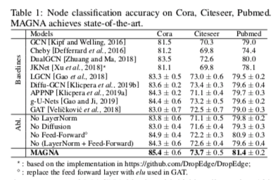
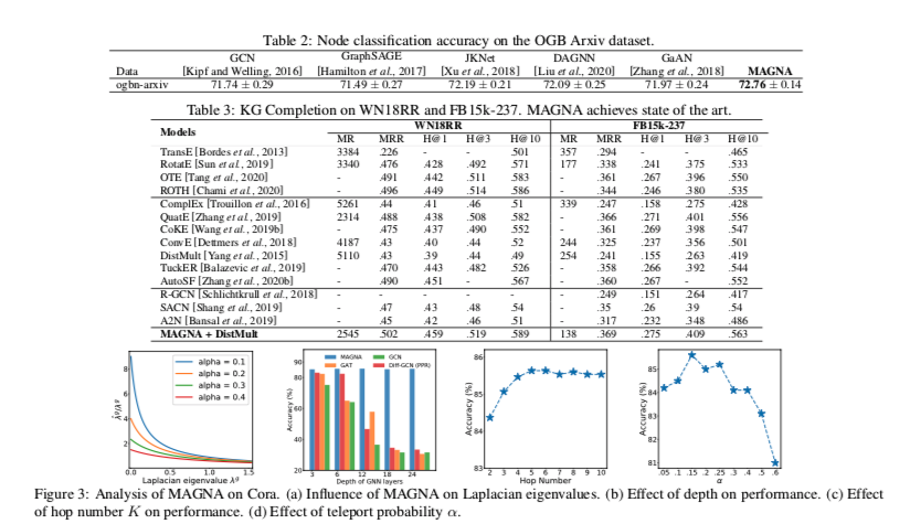
实验

Reviewer

The central question of the reviewers’ discussion was whether the contribution of this paper was significant enough or too incremental. The discussion emphasized relevant literature which already considers multi-hop attention (e.g. https://openreview.net/forum?id=rkKvBAiiz [Cucurull et al.], https://ieeexplore.ieee.org/document/8683050 [Feng et al.], https://arxiv.org/abs/2001.07620 [Isufi et al.]), and which should have served as baseline. In particular, the experiment suggested by R3 was in line with some of these previous works, which consider “a multi-hop adjacency matrix “ as a way to increase the GAT’s receptive field. This was as opposed to preserving the 1-hop adjacency matrix used in the original GAT and stacking multiple layers to enlarge the receptive field, which as noted by the authors, may result in over-smoothed node features. The reviewers acknowledged that there is indeed as slight difference between the formulation proposed in the paper and the one in e.g. [Cucurull et al.]. The difference consists in calculating attention and then computing the powers with a decay factor vs. increasing the receptive field first by using powers of the adjacency matrix and then computing attention. Still, the multi-hop GAT baseline of [Cucurull et al.] could be extended to use a multi-hop adjacency matrix computed with the diffusion process from [Klicpera 2019], as suggested by R3. In light of these works and the above-mentioned missing baselines, the reviewers agreed that the contribution may be viewed as rather incremental (combining multi-hop graph attention with graph diffusion). The discussion also highlighted the potential of the presented spectral analysis, which could be strengthened by developing new insights in order to become a stronger contribution (see R2’s suggestions).

Proposed methodology being more powerful than GAT is arguable:
When the attention scores for indirectly connected neighbors are still computed based on the immediate neighbors’ attention scores, it is not convincing enough to be argued as more powerful than GAT, which learns attention scores over contextualized immediate neighbors.Also, the approximate realization of the model described in Eqn: 5 follows a message-passing style to propagate attention scores. Suppose it is to be argued that standard message-passing-based diffusion is not powerful enough to get a good immediate neighbor representation that encodes neighbors’ information from far away. In that case, it is not immediately clear how a similar diffusion, when used for propagating attention scores from immediate neighbors to neighbors multiple hops away, will be more powerful.